16 Jul The basics of Excel

Essential concepts

Excel is organized as a table, containing rows, columns and their intersection: the cells. The rows are numbered, the columns are identified by a letter (for example the 3rd column is cell C). A cell is referred to by its column letter followed by its row number (E1 is the cell that crosses column E and the first row).

An Excel file is called a workbook which may include one or more worksheets. pvalue.io can only analyze the first worksheet

If a cell has not been formatted and the content of a cell is aligned on the left, it means that Excel recognizes this cell as text. If it is right-aligned, it can be a number or a date.

The formulas

The main advantage of Excel is that it is possible to perform a large number of operations from the cells (calculation of sums, means, and even statistical tests), using a simple syntax: the formulas. To understand how to use them, we suggest you visit the following page.

Frequent operations

Select a column

Click on the letter that identifies the column

Select a row

Click on the number that identifies the line

Delete a worksheet

1. Right click on the worksheet to be deleted
2. Delete

Delete a column

1. Right click on the column title (A, B, C, …)
2. Delete

Delete a row

1. >Right click on the row number
2. Delete

Filter one (or more) columns

The filter function is very convenient for this.

1. Select the column to filter
2. Click the Filter button
   
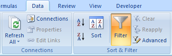
3. Select the desired categories

You can find more information on the following page (from Microsoft).

Change the cell format

Excel is able to recognize a large number of formats with different dates. Whether you enter 20/12/2015 or 20-12-2015 or 2015-12-20, Excel will understand that this is a date. In reality, the dates are stored as number of days since 1900-01-01 and then displayed according to the user’s default date format. Inconsistencies are often obtained; to resolve them, simply follow the following procedure:

1. Select the column
2. Right click > Cell format
3. Select the type of cell you want (e. g. date).

Copy a table and paste it on a new worksheet.

1. Left click on cell A1
2. Press the Shift key (⇧)
3. Keep pressing the Shift key and click on the cell at the bottom right of your data table.
4. Copy this table (Ctrl-C under Windows or ⌘-C on Mac)
5. Click on the new worksheet
6. Select Cell A1 of the new worksheet
7. Right click > Special Paste > Values
8. Click on OK

Transpose a table on a new worksheet

1. Click on the new sheet
2. Select Cell A1
3. Right click > Special Paste > Transposed
4. Click on OK

Insert a column

1. Click on the column title behind which you want to insert your new column
2. Right Click > Insert

Create a column from another column

1. Insert a column
2. Click on cell X2, X being the new column
3. Click on the formula bar
4. Enter the equal symbol (=)
5. Use the cell references. To do this you can:
   • Enter the formula straight away: for example, if you want X2 to be the sum of V2 and W2, then the formula to enter is : =V2+W2
   • Click on the cells to which you refer: on the previous example, click on the cell V2, then press the “+” key, then click on the cell W2

Extend the scope of a formula to all other rows in the column

If X2 is the cell that contains the formula, two options:

• Double click on the lower right corner of X2 (the cursor changes shape when you hover over this corner) to apply this formula to the entire column. This method is very convenient but will stop if there is missing data in a cell to which the formula refers
• Click on the bottom right corner, hold the click and move the cursor down the cell

Replace one value with another throughout the worksheet.

1. Ctrl-H (on Windows) or ⌘-H (on Mac)
2. In the “Search” field, enter the value to replace
3. In the “Replace” field, enter the replacement value (leave blank to obtain an empty cell)
4. Click on the “Replace All” button

Modify all the cells of a column that have the same value

1. Select the column
2. Ctrl-H (sur Windows) ou ⌘-H (sur Mac)
3. Click on Option, et in the Search box, sélectionnez “By colum”
4. Click on the “Replace All” button

Delete units in the columns of number

1. Select the column
2. Ctrl-H (on Windows) ou ⌘-H (on Mac)
3. In the “Search” field: write the unit
4. In the “Replace with” field: leave blank
5. Replace All

Exporting a file as Unicode Text

A Unicode Text file is a standardized file, in which the columns are separated by tabs and special characters are preserved. If your workbook has several worksheets, you must export them in text format one by one. It is not possible to export the entire workbook in text format.

1. Select the worksheet you want to export
2. Select “Save as…” from the “File” menu or on the icon, then click on “Other formats”
3. Select “Unicode text (*.txt)” as “File type”.